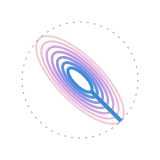
Gaussian layer

qkd.gaussian: an $N$-mode state is a mean $\overline{\mathbf{r}}\in {\mathbb{R}}^{2N}$ and a covariance $V\in {\mathbb{R}}^{2N\times 2N}$; every operation is a symplectic map or a Gaussian channel. Internal units and xpxp ordering throughout — Conventions.

from qkd import gaussian as g

States are immutable

Every operation returns a new State; sampling leaves the state unchanged. mean and cov are copies.

st = (g.Vacuum(2)
      .squeeze(0, r=0.8)
      .bs(0, 1, t=0.5)
      .thermal_loss(0, T=0.5, xi=0.01, ref="input"))

st.n_modes      # 2
st.physical()   # True
st.cov
# array([[ 0.402737,  0.      ,  0.141086,  0.      ],
#        [ 0.      ,  0.996629,  0.      , -0.698804],
#        [ 0.141086,  0.      ,  0.300474,  0.      ],
#        [ 0.      , -0.698804,  0.      ,  1.488258]])

Constructors

Constructor	Modes
Vacuum(n)	$n$
Coherent(x, p), Thermal(nbar), Squeezed(r)	1
Epr(r)	2
Moments(mean, cov)	$|\text{mean}|/2$

Covariances and means: reference states. No defaults.

Parameter	Unit	Range	Description
n	modes	$\ge 1$	Zero raises.
x, p	internal quadratures	finite	Displacement; $|\alpha {|}^2=(x^2+p^2)/2$.
nbar	photons	$\ge 0$, finite	$\overline{n}=0$ is the vacuum.
r	nepers	finite, unbounded	$r>0$ squeezes $\hat{x}$.
mean, cov	internal	—	Length $2N$ and $2N\times 2N$. Checked for finiteness, symmetry and the bona fide condition.

Epr(r) is two-mode squeezed vacuum: pure at every $r$, both symplectic eigenvalues $1/2$. Moments takes a covariance from elsewhere — a Fock state's Gaussian shadow, a measured matrix.

Symplectic operations

Method	Parameters	Effect
displace(mode, x=0.0, p=0.0)	quadratures, finite	mean shift only; covariance untouched
squeeze(mode, r)	$r$ in nepers, finite	$S=\mathrm{diag}(e^{-r},e^r)$ on that mode
rotate(mode, theta)	$\theta$ in radians, finite	phase-space rotation by $\theta$
bs(m1, m2, t)	$t\in [0,1]$, distinct modes	beamsplitter of transmittance $t$, not angle

Action	$V\mapsto SV{S}^{\mathrm{\top }}$ (form), preserving the bona fide condition — Gaussian · Ops
Checked	every mode index is bounds-checked; a beamsplitter given one mode twice raises
Closed intervals	bs(t), thermal_loss(T) and fock.State.loss(eta) accept $[0,1]$ inclusive; q.Channel(T), q.Fiber(T) and every detector eta require $(0,1]$ — same symbol, different admissible set

Thermal loss, and the required ref= plane

$$V⟼TV+[\frac{1-T}{2}+\frac{\xi }{2}\{\begin{array}{ll}T& \mathtt{\text{ref="input"}}\\ 1& \mathtt{\text{ref="output"}}\end{array}]{\mathbb{1}}_2$$

Vacuum through the loss port, then excess noise. Pure loss is $\xi =0$.

Parameter	Unit	Default	Description
mode	—	required	Which mode the channel acts on.
T	—	required	Transmittance $T\in [0,1]$.
xi	SNU	0.0	Excess noise $\xi \ge 0$ at the plane ref names. The one argument here not in internal units: halved on the way in (SNU boundary).
ref	—	required, keyword-only	"input" or "output". Required even at $\xi =0$.

g.Vacuum(1).thermal_loss(0, T=0.5, xi=0.01)
# TypeError: State.thermal_loss() missing 1 required keyword-only argument: 'ref'

g.Vacuum(1).thermal_loss(0, T=0.5, xi=0.01, ref="bob")
# ValueError: ref must be 'input' or 'output'

One channel, either plane:

a = g.Vacuum(1).thermal_loss(0, T=0.4, xi=0.02,  ref="input")
b = g.Vacuum(1).thermal_loss(0, T=0.4, xi=0.008, ref="output")

a.cov[0, 0] == b.cov[0, 0]      # True -- 0.504

Gaussian · Loss pins that identity, the vacuum fixed point, the $\sqrt{T}$ amplitude scaling and physicality under positive $\xi$.

Measurement

Sampling is repeated-preparation: i.i.d. draws, state unchanged.

x = g.Coherent(1.0, 0.0).homodyne(0, angle=0.0, shots=100_000, seed=3)
x.shape, x.mean(), x.var()
# ((100000,), 0.9986, 0.5020)     -- mean 1, variance 1/2

h = g.Vacuum(1).heterodyne(0, shots=100_000, seed=1)
h.shape, h.var(axis=0)
# ((100000, 2), array([0.9958, 0.9947]))

Method	Parameters	Returns
homodyne(mode, angle=0.0, shots=1, seed=0)	$\theta$ in radians, finite	(shots,) outcomes of ${\hat{x}}_{\theta }=\hat{x}\cos \theta +\hat{p}\sin \theta$
heterodyne(mode, shots=1, seed=0)	—	(shots, 2), drawn from the Husimi distribution
condition(mode, angle, outcome)	radians, internal quadrature	the remaining $N-1$ modes, conditioned

Buffers	owned by the array
Heterodyne	samples the covariance plus one vacuum unit from the balanced splitter, so vacuum reads variance $1$ per quadrature, not $1/2$: the 3 dB penalty
seed	default 0; the same seed reproduces the samples

Conditioning

Homodyne on one mode — Schur complement with a pseudo-inverse — which removes that mode:

c = g.Epr(1.0).condition(1, 0.0, 0.7)

c.n_modes       # 1
c.cov[0, 0]     # 0.132901  == 1 / (2*cosh(2)), below the vacuum 1/2
c.mean[0]       # 0.674819  == tanh(2) * 0.7

The sub-vacuum $x$ variance is EPR steering. Point-to-point Gaussian modulation never calls this; the relay topologies do.

CV toolbox

Closed Gaussian forms, no numerical integration.

Method	Returns
wigner(mode, xs, ps)	Wigner grid, shape (len(ps), len(xs))
husimi(mode, xs, ps)	Husimi $Q$ on the same grid
keep(modes) / drop(modes)	partial trace, order preserved; keep needs at least one mode and rejects duplicates
evolve(G, t)	unitary evolution under $H=\frac{1}{2}{\mathbf{r}}^{\mathrm{\top }}G\mathbf{r}$; G symmetric and $2N\times 2N$, else ValueError
purity()	$1/(2^n\sqrt{detV})$
entropy()	von Neumann entropy in bits
spectrum()	symplectic eigenvalues, internal units, ascending
negativity()	Wigner-negativity volume, 0.0
physical(atol=1e-9)	the bona fide check
overlap(other)	Hilbert–Schmidt overlap $\mathrm{Tr}(\rho \sigma )$
fidelity(other)	fidelity, squared convention
trace_distance(other)	$\frac{1}{2}\Vert \rho -\sigma {\Vert }_1$, pure pair only
trace_bounds(other)	$(1-\sqrt{F},\sqrt{1-F})$

xs and ps each need at least two finite, strictly increasing points.

Wigner and Husimi

$$W(\mathbf{d})=\frac{\exp (-\frac{1}{2}{\mathbf{d}}^{\mathrm{\top }}{V}^{-1}\mathbf{d})}{2\pi \sqrt{detV}},Q=W{|}_{V\to V+\frac{1}{2}\mathbb{1}}$$

Both normalised in $dxdp$ on the named mode's reduced state. Heterodyne samples $Q$.

import numpy as np

xs = ps = np.linspace(-5, 5, 201)
W = g.Coherent(1.5, -0.5).wigner(0, xs, ps)

W.sum() * (xs[1] - xs[0]) * (ps[1] - ps[0])   # 1.0000
W.max()                                        # 0.31831 == 1/pi

$Q$ peaks at $1/(2\pi )$, half the Wigner peak, and $0\le Q\le 1/(2\pi )$ since $det(V+\frac{1}{2}\mathbb{1})\ge 1$. That is the $dxdp$ bound; the usual $1/\pi$ is the $d^2\alpha$ normalisation, the factor 2 being the Jacobian. Toolbox · Phase space.

Partial trace and entanglement

e = g.Epr(0.8)

e.entropy()               # 0.0        -- globally pure
e.keep([0]).entropy()     # 1.77069    -- entanglement entropy
e.keep([1]).cov[0, 0]     # 1.288732   == cosh(1.6) / 2

Half an EPR pair is Thermal(sinh(r)**2). drop([0]) is keep([1]).

Evolution under a quadratic Hamiltonian

$S=\exp (\mathrm{\Omega }Gt)$, $G$ symmetric, xpxp. The $xp$ generator squeezes:

G = np.array([[0.0, 1.0], [1.0, 0.0]])
ev = g.Vacuum(1).evolve(G, 0.3)

ev.cov[0, 0], ev.cov[1, 1]   # 0.911059, 0.274406  == e^0.6/2, e^-0.6/2
ev.purity()                  # 1.0 -- unitary, so purity is preserved

Purity, entropy, spectrum

$$\mu =\frac{1}{2^n\sqrt{detV}},S=\sum _{k}G\left(\frac{2{\nu }_k-1}{2}\right),G(x)=(x+1){\log }_2(x+1)-x{\log }_{2}x$$

${\nu }_k$: moduli of the eigenvalues of $i\mathrm{\Omega }V$, one per mode, internal units — vacuum $0.5$, pure iff every ${\nu }_k=0.5$. The $2{\nu }_k$ is the SNU boundary.

th = g.Thermal(0.5)

th.spectrum()    # array([1.])
th.purity()      # 0.5      == 1 / (2*nbar + 1)
th.entropy()     # 1.377444 == 1.5*log2(1.5) - 0.5*log2(0.5)

spectrum()'s ceiling
Refusal	a surviving imaginary part is refused, $i\mathrm{\Omega }V$ having real spectrum for any bona fide $V$
Threshold	the backward error of a general eigensolve, $\epsilon \Vert i\mathrm{\Omega }V\Vert$: it scales with $max|V|$, while the bona fide slack stays absolute
First refusal	$r=8.17$, where the answer is already wrong by $3.2\times {10}^{-3}$
Epr's own limits	bona fide refusal from $r=8.45$, f64 ceiling at $r=9.2$
Usable range	treat $r>8$ as unusable whether or not it raises. A link's covariance entries are in the tens

Distinguishability

$$\mathrm{Tr}(\rho \sigma )=\frac{\exp (-\frac{1}{2}{\mathbf{d}}^{\mathrm{\top }}(V_1+V_2{)}^{-1}\mathbf{d})}{\sqrt{det(V_1+V_2)}},\mathbf{d}={\overline{\mathbf{r}}}_1-{\overline{\mathbf{r}}}_2$$

Method	Exactness
overlap	closed form at every $N$, no matrix square root; equals purity() when the states coincide
fidelity	squared, $F={\left(\mathrm{Tr}\sqrt{\sqrt{\rho }\sigma \sqrt{\rho }}\right)}^2$: a pure pair gives $|⟨\psi |\varphi ⟩{|}^2$, two coherent states sit $e^{-|\alpha -\beta {|}^2}$ apart. Closed at one mode; for $N>1$ exact when either state is pure, and a mixed $N>1$ pair is refused

a, b = g.Coherent(1.0, 0.0), g.Coherent(0.0, 0.0)   # alpha = 1/sqrt2 and 0

a.overlap(b), a.fidelity(b)   # 0.606531, 0.606531  == exp(-|alpha|^2) = exp(-1/2)
a.trace_distance(b)           # 0.627271  == sqrt(1 - F), both pure
g.Thermal(0.5).trace_distance(g.Thermal(1.0))
# NotImplementedError: trace distance is exact here only for a pure pair

Trace distance
No general closed form	set by the eigenvalues of $\rho -\sigma$, which the moments do not fix
trace_distance	pure pair only, $\sqrt{1-F}$; refuses otherwise
trace_bounds	$1-\sqrt{F}\le D\le \sqrt{1-F}$ for every pair, equality at the upper end where trace_distance answers
Thermal(0.5) vs Thermal(1.0)	$F=0.951918$, $D\in [0.024337,0.219275]$ — a bound, not an estimate

Negativity

negativity() returns $\int |W|-1$ as 0.0: by Hudson's theorem a Gaussian Wigner function is non-negative, so no grid is integrated. A Fock-layer volume on a coherent, squeezed or thermal state therefore measures truncation.

Derived states

keep, drop and evolve return an ordinary State through Moments' constructor — every method, in any order — re-checking finiteness, symmetry and the bona fide condition.

sub = g.Epr(0.8).keep([0])

sub.entropy()                       # 1.77069
sub.thermal_loss(0, T=0.5, xi=0.0, ref="input").cov[0, 0]   # 0.894366
sub.homodyne(0, shots=3, seed=1)    # array([-0.032070, -1.209714, -0.258740])